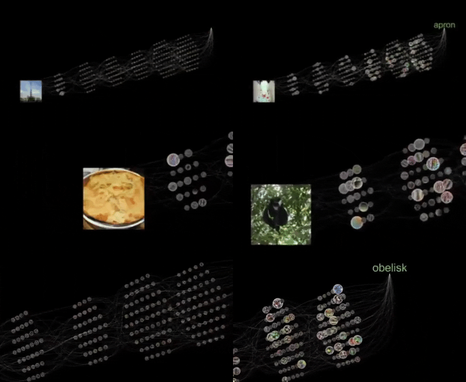
When our eyes see an image, various receptors in the retina respond by firing. Some fire in response to various colours. Some fire in response to light and shadow. Imagine that these cells are arranged in layers. If those simple cells in the first layer fire, they pass a signal to the next layer up. The cells in that layer might only fire if they get enough ‘activations’ from the previous layer. Each layer in turn receives the input of more and more complicated patterns of connections from the previous layer. Eventually, the brain receives the signal.
A biologist might read that paragraph, and shudder. Neural networks have long been around in the field of artificial intelligence, and they’ve been modelled after that simple analogy. Since about 2012 or so, the field of neural networks has exploded with the raw computing power of commercial grade GPUs. The key to the recent explosion has been this combination of raw computing power, large million image datasets, and the idea of allowing inputs to back propogated along the network: basically, if you put enough images of a dog in front of the neural network, the average pattern of connection and firing could be labelled ‘dog’; then if a picture of, say, a cat was put in front of the network, the distance or similarity of the firing could be compared to that we know for ‘dog’ and a score computed. Put enough pictures of cats in front of the neural network, and the network learns what ‘cats’ look like.
I simplify enormously, of course, but that’s the gist. The neat thing is, once you’ve got a network trained on thousands of different kinds of things - which takes enormous computing power and resources - you can retrain just the last layer of the network with new data, to teach it what something looks like that it wasn’t trained on. Retrain the network on pictures of Roman pottery, and it will learn what different kinds of Roman pottery look like (but you can’t use it for dogs any more). The network lights up in a particular way when it encounters pictures of verenice nera, and we can say: this pattern = verenice nera, with a given probability.
(For a discussion on the use of neural networks in archaeology, see Baxter 2014).
Indeed, you don’t even need to have labelled categories of things for a pretrained neural network to be useful. The Yale DH Lab uses a neural network without that final layer to find image similarity: it shows images to the network, and computes the distance between how the network lights up for one image versus a different image. This distance can then be expressed in two-dimensional space, and you end up with a visualization of visual similarity!
The two ipynb files in the week 7 workbench walk you through an image classifier, and image similarity, using a dataset from POTSHERD: The Atlas of Roman Pottery. Do the image-classifier.ipynb as it also contains the code to grab the data.
Try going further by swapping in your own images! What kinds of archaeological things might we want to do now that we have this ability? Go to openalex.org and search out what archaeologists are up to in this domain (and you might also take a peak at the Vesuvius Challenge, which uses technologies that have their roots in what you’re doing this week.)