👋🏻 Hi!
Let’s do some coding. The interface below accepts python code (it might take a moment to load up; if you can see a ‘play’ etc it’s loaded). Try copying and pasting this:
text = "Oh yeah, digital archaeology!"
print(text)
into the gray box at the bottom of the interface below. Then, hit shift+enter while your cursor is in the box:
Now try this:
one = 1
two = 2
print(one + two)
See how easy that was? You just entered some python code into a coding environment powered by a version of the Python language. That gray box is a ‘cell’ powered by the Jupyter lab interface. When you hit shift+enter (or hit the ‘play’ arrow) the code is passed to an interpreter which translates the python language into something your machine understands.
We want to get something similar set up on your computer. In this course, we will use the Python and R languages for the most part, so we need to get an interpreter or ‘kernel’ for Python and for R installed. We’ll start with Python, for now.
Installing Python directly onto your machine can be a pain though, since there are so many of you and so many different computers y’all might have. We will be using, for parts of the course, an application called ‘Jupyter Lab Desktop’ that ought to make life easier for us. I have created an extension for Jupyter Lab Desktop that lets us not only do computational analysis, but also, make wiki-style notes around our readings and our analyses (following ‘personal knowledge management’ approaches.)
Part One: Get The Content for our Lab Bench
I have made a folder with a variety of notes (plain text files that use the .md file extension to signal that I’m using markdown to indicate headers, bullets, and so on) and python ’notebooks’ that mix python code with markdown comments. These files are signaled with the .ipynb extension, and they can be understood and run by Jupyter.
The attraction for us is that we can make notes using markdown, and we can treat the .ipynb files like experiments that we link into our thinking.
Your first task then is to right-click and open this link in a new browser tab: https://github.com/shawngraham/digiarch-labbench.
Then click on the green ‘Code’ button so you can click ‘Download zip.’
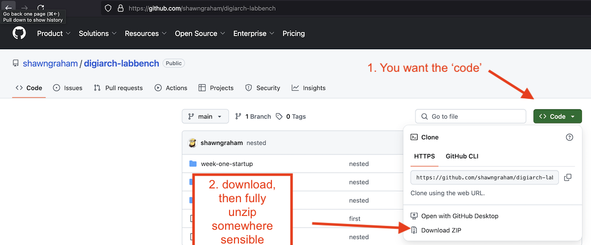
Unzip this file in a location on your computer that is easy to find.
Part Two: Our Lab Bench
We will use JupyterLab Desktop as our lab bench for analytical code work and note taking. It provides a clean, self-contained environment that will not interfere with any other software on your computer. First of all, grab the version that works on your machine:
-
Install for Windows using this file
-
Install for Mac using this file (if you have an older Mac from before Apple Silicon chips were introduced, ie 2020, try this instead)
-
Install for Linux have some options depending on which variety of Linux.
Now we will install the specific Python libraries and extensions needed for this course with a single command.
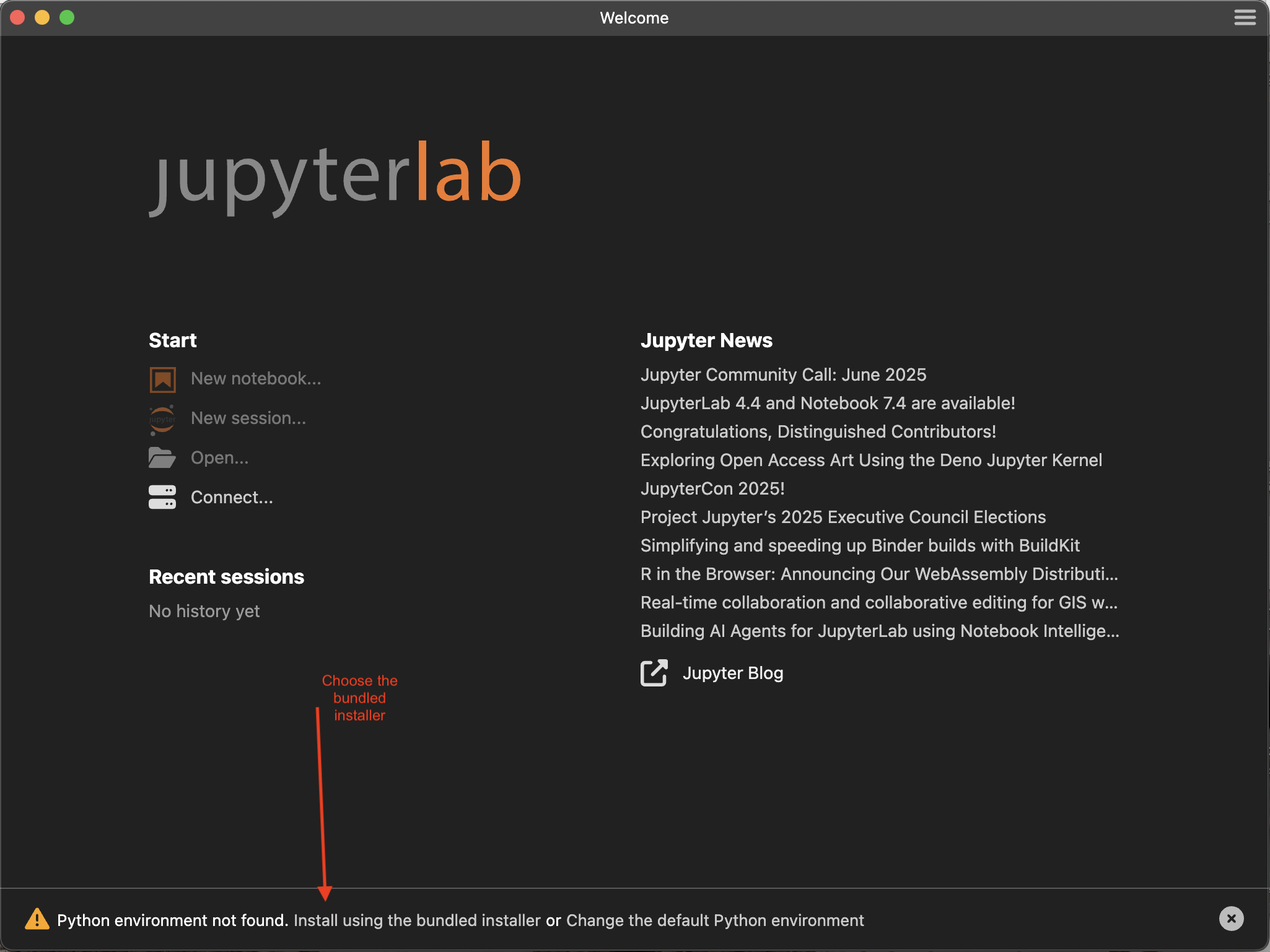
Step 1. When you first install Jupyter, it will check to see if you have Python installed on your machine. If it cannot find it in the usual places, it will ask you if you want to install with the bundled Python. In the screenshot below it’s not clear that where it says ‘Install using the bundled installer’ is actually a link. It is! Click on that. This might take four or five minutes.
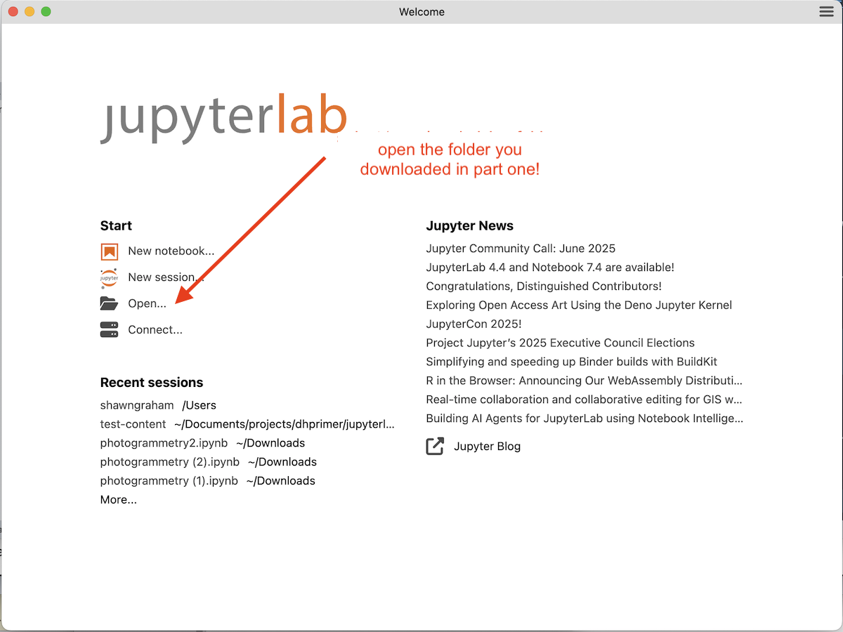
Step 2. When it’s done, the install notification will disappear and the main splash screen will be showing. Select ‘open’ and choose the lab bench folder you downloaded and unzipped. This is where you want to do your course work.
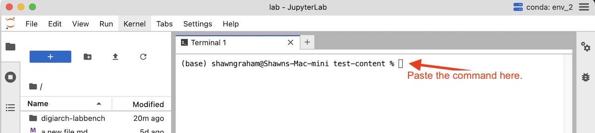
Step 3. Once it loads, go to the top menu bar and click: File > New > Terminal
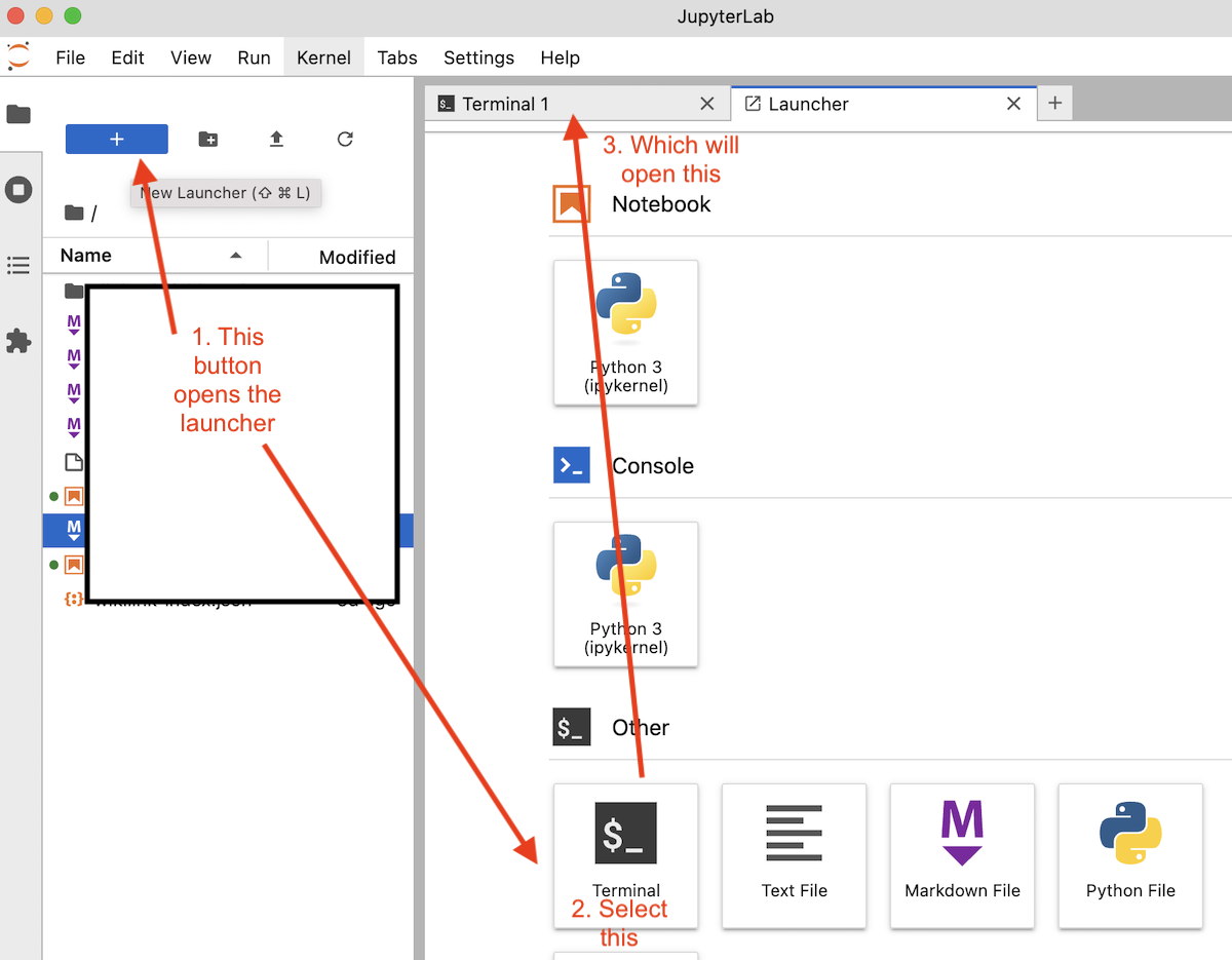
Step 4. A command-line terminal will open inside a new JupyterLab tab. It will have a prompt like $ or > or even %.
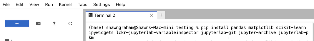
Step 5. Copy the entire command below from pip all the way to jupyterlab-pkm. The command pip is used to obtain little pieces of pre-packaged code. Pip will download and then install a number of extensions for python and jupyter that we need. It is installing them into the version of python indicated in the top right-hand corner of the interface.) So double-click the command below to select all of it, then copy (Ctrl+C or Cmd+C).
pip install pandas matplotlib scikit-learn ipywidgets lckr-jupyterlab-variableinspector jupyterlab-geojson jupyter-archive jupyterlab-pkm
Step 6. Paste the command into the JupyterLab terminal (Ctrl+V or Cmd+V) and press Enter.
You will see a lot of text as that command runs and packages are downloaded and installed. This may take a few minutes. Wait for it to finish and for the command prompt ($ or >) to reappear.
Step 7. Completely close JupyterLab Desktop.
Step 8. Re-open JupyterLab Desktop. This refreshes the program with the new functionality you just downloaded. Select ‘open’ and find the digiarch-labbench. Select it. (It should also be listed under ‘Recent Sessions’ and you can click on it there.) If you see the PKM extension pop-up when you open the folder, then you’re good to go! You can also check that it’s working by clicking view -> Activate Command Palette -> and then typing PKM: and you should see a list of commands (eg: PKM: Build/Rebuild Wiki Index).
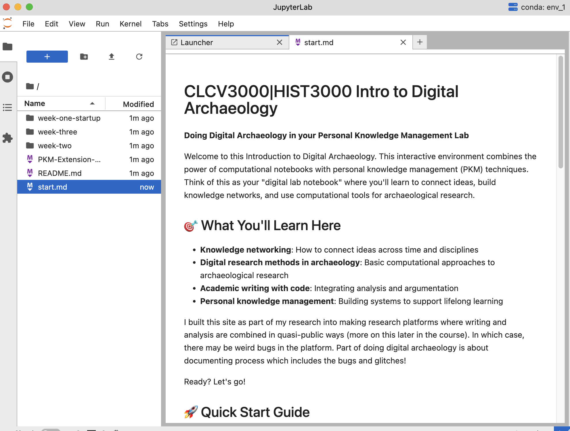
I have preloaded this folder with guidance on note-making, and a number of computational notebooks (which are signaled by having the .ipnyb at the end of the filename) which we will use throughout the course.
- Explore the existing materials,
- try to make some notes on your readings, your observations, hiccups or roadblocks you’ve encountered this week.
- Make reflection note and your wk-1 memo note in the environment. Then right-click on those notes in the file pane and select ‘download’ for those two notes. Then upload those notes to your github repository.
Video Walk Throughs
These video walkthroughs use a generative AI to turn my words into a transcript. I see that they also try to allow question and answering in a wee ‘assistant’ chat box. Such ‘answers’ are probabilistic token predictions, and NO ANSWER so-generated constitutes an actual answer: ASK ME DIRECTLY if you have questions. (That’s what I get for going with a free screen-capture video service, sigh.)
and
How to take screenshots I mention in that video about taking screenshots if you need help. A good screenshot shows me what you were trying to do and the result (make a series if you have to - scroll, screenshot, scroll, new screenshot… etc). Windows Users - here are some ways to do it. Mac users: cmd + 4 will let you define a square of the screen to take a picture of; cmd + 5 will do the same thing for a quick movie.
Help, this isn’t working for me.
That said, AS AN ALTERNATIVE, or if you run into trouble using this application, you may download all of the course materials from this link and use Obsidian to manage your note making, and then open the ipynb files directly in the https://colab.research.google.com/ service under ‘file -> upload notebook’.